#008 🍵 Matcha DAX Break – Smart Ways to Practice DAX

’Matcha DAX Break’ is a deliberate learning ritual — a moment to slow down, focus, and consistently practice DAX skills beyond daily work demands. ⭐

How to practice DAX when your job doesn’t really require it (yet)

One of the most common things I hear from people learning DAX is:

“I understand the basics, but I don’t really use advanced DAX at work, so I don’t know how to practice.”

And honestly? That’s a very real problem.

If your daily reports are based on simple visuals and basic measures, you rarely need more complex DAX.
But at the same time — you want to grow, you want to understand context, filters, and performance… and eventually feel confident calling yourself a Power BI Developer.

That’s exactly why I’m starting Matcha DAX Break ☕

Grab the dataset and the guide today to follow along with me and master these DAX patterns through hands-on practice.

🌱 My philosophy of learning DAX

Instead of waiting for “perfect business use cases”, I focus on intentional practice.
Here are two approaches I strongly believe in:

1️⃣ One measure — many ways

Take a single business question and try to answer it using different DAX patterns.

• CALCULATE + FILTER
• Variables
• Iterators vs simple aggregations
• ALL vs ALLSELECTED vs ALLEXCEPT

Then:

• Compare results
• Observe behavior in a table
• Analyze filter context step by step

This helps you understand why DAX works — not just that it works.

👉 Example 1: Total Sales of the Highest-Spending User per Country

It is interesting because it requires filtering, aggregation, and understanding of context.

To get the most out of this lesson, create the measures listed below within the _Metrics table. Once ready, set them up in a Matrix visual. Start by analyzing the results per country, then try swapping the country for users[id] to see how the numbers shift.

Ask yourself: What results are we getting and why?

For an advanced 'Vigilance’ test, try replacing VALUES with ALL in the V2 and V3 measures. Observe the change in behavior—investigating why this happens is the best way to truly master the mechanics of Filter Context!

Here are 3 approaches worth showcasing:

1. The „Old School” Way (Filter & Table Scan)

This approach is very common for beginners. It iterates through all users and checks if their total transaction amount matches the maximum one found in the list.

TopSpenderSales_V1 = 
CALCULATE(
    SUM(transactions[amount]),
    FILTER(
        ALL(users[id]),
        [Total Amount] = MAXX(ALL(users[id]), [Total Amount])
    )
)

Total Amount = SUM(orders[amount])

Why it’s „Old School”: It relies on FILTER and MAXX over a potentially large table (users). It is easy to understand but heavy on CPU.

2. The „Context Transition” Way (TOPN)

This is much more elegant. It uses TOPN to create a virtual table containing only the single user with the highest sales.

TopSpenderSales_V2 = 
VAR TopUser = TOPN(1, VALUES(users[id]), [Total Amount], DESC)
RETURN
CALCULATE(
    SUM(transactions[amount]),
    KEEPFILTERS(TopUser)
)

Vigilance Note: As we discussed, if two users have the exact same transaction total, TOPN(1, ...) will return both. Your result will be the sum of both users’ transactions. To fix this, you would add users[id], ASC as a tie-breaker inside TOPN.

3. The „Modern & Optimized” Way (TREATAS)

This is the highest performance level. It retrieves the ID of the top spender and „maps” it directly onto the relationship between users and transactions.

TopSpenderSales_V3 = 
VAR TopUserId = TOPN(1, VALUES(users[id]), [Total Amount], DESC)
RETURN
CALCULATE(
    SUM(transactions[amount]),
    TREATAS(TopUserId, users[id])
)

Why it’s „Expert”: TREATAS is often faster than standard filter passing because it treats the virtual table result as if it were a direct physical filter on the users[id] column.

2️⃣ From SQL to DAX (real-model approach)

This is where things get really interesting.

In this paragraph, instead of creating artificial visuals, I practice DAX on existing data models by:

• Taking a SQL query (with joins, group by, filters).
• Rebuilding the same logic as a DAX query.
• Understanding how relationships and filter context replace joins.

This approach:

• Feels much more real.
• Is perfect for people coming from SQL.
• Builds strong mental models of how DAX actually thinks.

You stop asking “Which function should I use?”
And start asking “What is the filter context here?”

🌱Many learners jump straight into writing measures.

Before asking:

“How do I calculate this?”

I want you to ask:

“What table do I need first?”

In this category, the focus is on:

• returning tables with DAX queries
• understanding what each step produces
• and treating DAX like a transformation pipeline

👉 This is where I start from a basic table and gradually shape it — before turning anything into a final DAX query.

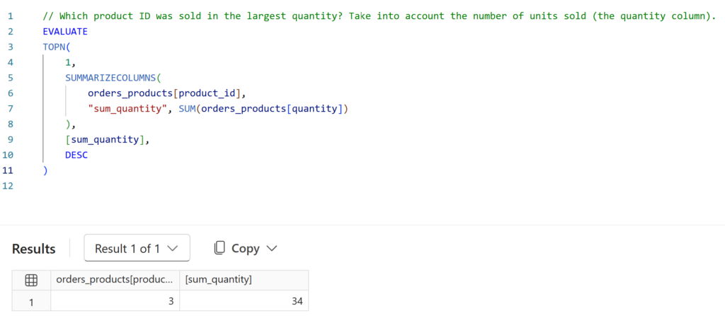
👉 Example 1: Which product ID was sold in the largest quantity? Take into account the number of units sold (the quantity column).

👟 Step 1: We start by checking which table the data will come from, so we look at the model in Power BI in Model view and examine which table contains the quantity column. In our case, the data comes from the orders_products table.

We begin by loading the main table, which creates the evaluation context — a table where we aggregate quantity values by product_id.
In SQL, this would be done using GROUP BY, while in DAX the same logic is handled more efficiently with the SUMMARIZECOLUMNS function.

\\Main view in SQL query
SELECT product_id, SUM(quantity) AS sum_quantity
FROM orders_products
GROUP BY product_id

\\DAX query
EVALUATE
SUMMARIZECOLUMNS (
    orders_products[product_id],
    "sum_quantity", SUM ( orders_products[quantity] )
)

As a result, we get a table with two columns: product_id and total quantity.
👟 Step 2: Next, we sort the table and extract the row with the highest value.

Next, to achieve this in DAX, we use the TOPN function and select the first row (1) from the given context — our table — sorting by the sum_quantity column in descending order.

\\SQL query
SELECT TOP 1
	product_id, 
	SUM(quantity) AS sum_quantity
FROM orders_products
GROUP BY product_id
ORDER BY sum_quantity DESC

\\DAX query
EVALUATE
TOPN(
    1,
    SUMMARIZECOLUMNS(
        orders_products[product_id],
        "sum_quantity", SUM(orders_products[quantity])
    ),
    [sum_quantity],
    DESC
)

👉 Example 2: List the top two cities with the highest number of users.

👟 Step 1: We start by checking which table the data will come from, so we look at the model in Power BI in Model view and examine which table contains the city and users id column. In our case, the data comes from the users table.

\\Main view in SQL query
SELECT city, count(*) AS cnt_users
FROM users
GROUP BY city

\\DAX query
EVALUATE
	SUMMARIZECOLUMNS(
		Users[city],
		"cnt_users", DISTINCTCOUNT(Users[id])
	)

As a result, we get a table with two columns: city and total cnt_users.
👟 Step 2: Next, we sort the table and extract 2 rows with the highest value.

\\Main view in SQL query
SELECT TOP 2
       city,
       COUNT(*) AS cnt_users
FROM users
GROUP BY city
ORDER BY cnt_users DESC;

\\DAX query
EVALUATE
TOPN(
    2,
    SUMMARIZECOLUMNS(
        Users[city],
        "cnt_users", DISTINCTCOUNT(Users[id])
    ),
    [cnt_users],
    DESC
)

🐛 Trust, but Verify: The Hidden Traps of SQL/DAX

First of all, we could build this query using SUMMARIZE, but it wouldn’t be efficient. We would be forced to use CALCULATE to trigger context transition manually, adding unnecessary complexity to the engine’s work.

EVALUATE
TOPN (
    2,
    ADDCOLUMNS (
        SUMMARIZE ( Users, Users[city] ),
        "cnt_users", CALCULATE ( DISTINCTCOUNT ( users[id] ) )
    ),
    [cnt_users], DESC
)

Quick Guide: SUMMARIZE vs. SUMMARIZECOLUMNS

• Use SUMMARIZECOLUMNS for Queries: It is the gold standard for EVALUATE statements. It’s faster, cleaner, and handles CALCULATE automatically. Rule: Use it for standalone tables and data exports.
• Use SUMMARIZE for Measures: Use it only for grouping columns within a measure. To add calculations, always wrap it in ADDCOLUMNS. Rule: Use it when your code must respect report slicers and filters.

The Bottom Line: Be vigilant. A query that works isn’t always a query that’s optimized. In high-volume data, the wrong choice can lead to massive performance hits.

⚠️The second trap lies in the query results: instead of two rows, the DAX query correctly returns four. This happens because three countries share the exact same number of users. In my opinion, it is correct to include all of them in the table to maintain data integrity.

However, in the real world, a stakeholder might insist on seeing exactly two rows (for example, to fit a specific UI design). If you are asked to force a limit and break the tie, you need to provide the engine with a second sorting criteria.

EVALUATE
TOPN(
    2,
    SUMMARIZECOLUMNS(
        Users[city],
        "cnt_users", DISTINCTCOUNT(Users[id])
    ),
    [cnt_users], DESC,   -- Primary criterion.
    Users[city], ASC     -- Secondary criterion (alphabetical - tie-breaker)
)

🎯 The goal of Matcha DAX Break

In conclusion, this is not about memorizing functions.

It’s about:

• Thinking in DAX
• Practicing without pressure
• Growing even if your current job doesn’t demand it

Short breaks.
Focused exercises.
One sip of matcha at a time 🍵

Moreover, If you’re learning DAX for the future version of your career — this space is for you.